# 算法图解
# 选择排序
# 复杂度
选择排序是一种灵巧的算法,速度不是很快 快速排序更快 运行时间为 O(nlogn)
# 算法
# Finds the smallest value in an array
def findSmallest(arr):
    # Stores the smallest value
    smallest = arr[0]
    # Stores the index of the smallest value
    smallest_index = 0
    for i in range(1, len(arr)):
        if arr[i] < smallest:
            smallest = arr[i]
            smallest_index = i
    return smallest_index


# Sort array
def selectionSort(arr):
    newArr = []
    for i in range(len(arr)):
        # Finds the smallest element in the array and adds it to the new array
        smallest = findSmallest(arr)
        # 这里会从arr中弹出这个最小的,加入到新的数组中
        newArr.append(arr.pop(smallest))
    return newArr


print(selectionSort([5, 3, 6, 2, 10]))
# 什么是递归?
递归,就是自己调用自己
# 什么是调用栈?
计算机在内部使用被称为调用栈的栈 假设你调用greet("maggie"),计算机将首先为该函数调用分配一块内存。

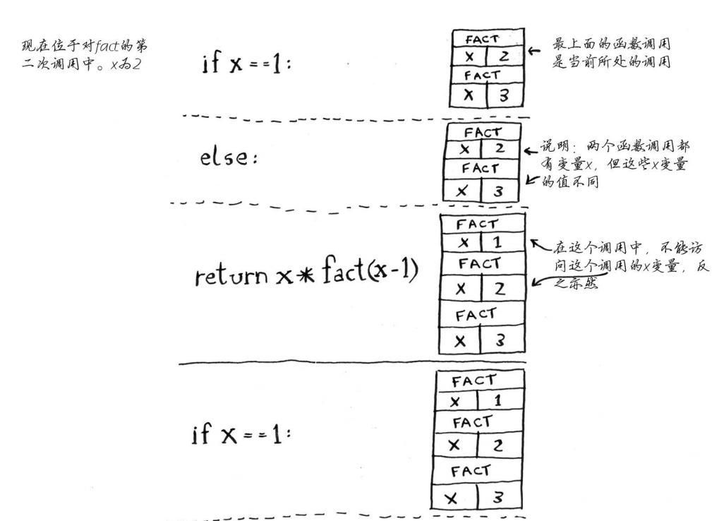
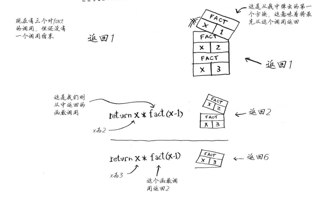
 函数返回的时候 ,栈顶内存被弹出
当你调用函数greet2时,函数greet只执行了一部分。这是本节的一个重要概念: 调用另一个函数时,当前函数暂停并处于未完成状态 你就从函数greet返回。这个栈用于 存储多个函数的变量,被称为调用栈。
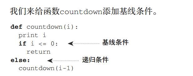
阶乘递归函数:
def fact(x):
if x == 1:
return 1
else:
return x * fact(x-1)
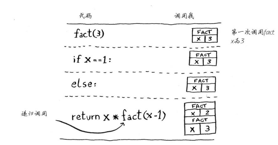
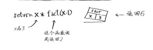
每个fact调用都有自己的x变量。 在一个函数调用中不能访问另一个的x变量。
栈有两种操作:压入和弹出。 所有函数调用都进入调用栈。 调用栈可能很长,这将占用大量的内存。
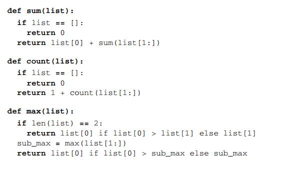
递归求和、求count、获取最大值
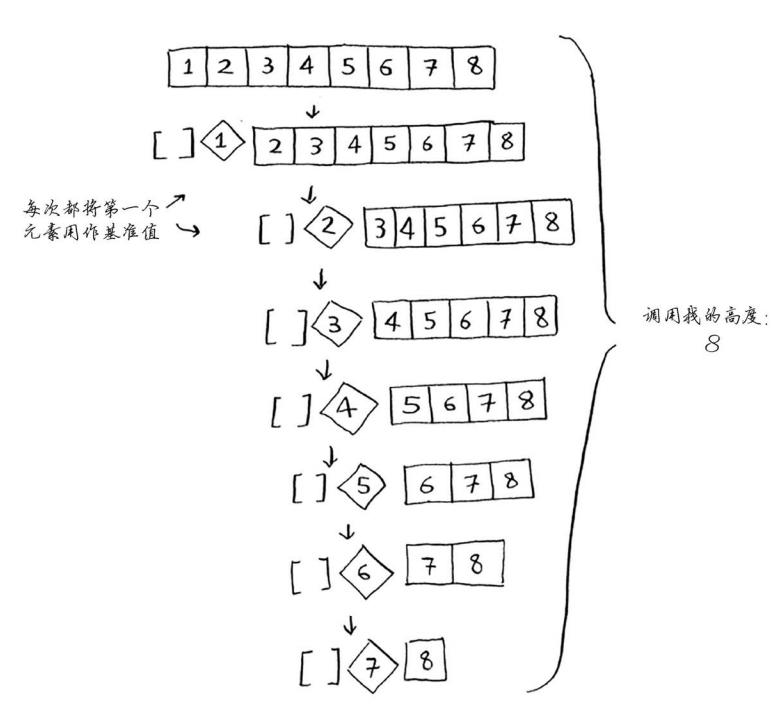
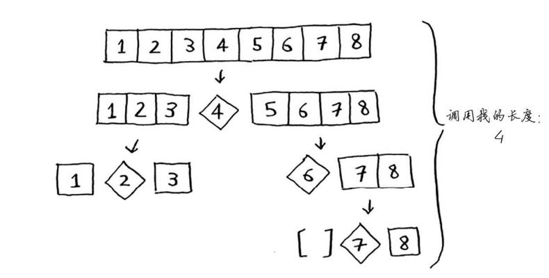
# 什么是分而治之(Divide and conquer, D&C)?
分而治之是你学习的第一种通用的问题解决方法 一种著名的递归式问题解决方法。
分而治之工作原理:
- 找出简单的基线条件,必须尽可能的简单
- 不断将问题分解(缩小规模) 知道符合条件
递归求和
def sum(list):
  if list == []:
    return 0
  return list[0] + sum(list[1:])
递归方式实现的二分查找
l = [2, 3, 5, 10, 15, 16, 18, 22, 26, 30, 32, 35, 41, 42, 43, 55, 56, 66, 67, 69, 72, 76, 82, 83, 88]


def find(l, aim, start=0, end=None):  #
    end = len(l) if end is None else end  # 让下面传上来的元素个数不改变初始的元素个数
    mid_index = (end - start) // 2 + start  #
    if start <= end:
        if l[mid_index] < aim:
            return find(l, aim, start=mid_index + 1, end=end)
        elif l[mid_index] > aim:
            return find(l, aim, start=start, end=mid_index - 1)
        else:
            return mid_index
    else:
        return '找不到这个值'


ret = find(l, 3)
print(ret)
# 常用算法
# 二分查找算法
def binary_search(list, item):
    # low and high keep track of which part of the list you'll search in.
    low = 0
    high = len(list) - 1

    # While you haven't narrowed it down to one element ...
    while low <= high:
        # ... check the middle element
        mid = (low + high) // 2
        guess = list[mid]
        # Found the item.
        if guess == item:
            return mid
        # The guess was too high.
        if guess > item:
            high = mid - 1
        # The guess was too low.
        else:
            low = mid + 1

    # Item doesn't exist
    return None


my_list = [1, 3, 5, 7, 9]
print(binary_search(my_list, 3))  # => 1

# 'None' means nil in Python. We use to indicate that the item wasn't found.
print(binary_search(my_list, -1))  # => None
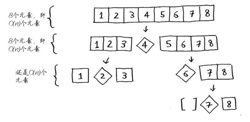
# 快速排序
复杂度 O(nlogn), 使用递归,数组分解,从数组选择第一个元素,成为基准值(pivot),第一个元素作为基准值,找出比基准值大的元素。 被成为分区,现在有三个部分组成
- 小于基准值的数组
- 基准值
- 大与基准值的数组
最糟情况 O(n^2)
最佳情况O(nlogn)
最佳情况也是平均情况,每次随机选择一个数组元素作为基准值哟
def quicksort(array):
  if len(array) < 2:
    # base case, arrays with 0 or 1 element are already "sorted"
    return array
  else:
    # recursive case
    pivot = array[0]
    # sub-array of all the elements less than the pivot
    less = [i for i in array[1:] if i <= pivot]
    # sub-array of all the elements greater than the pivot
    greater = [i for i in array[1:] if i > pivot]
    return quicksort(less) + [pivot] + quicksort(greater)

print(quicksort([10, 5, 2, 3]))
# 散列函数
- 包含额外逻辑的数据结构,使用散列函数来确定元素的存储位置
- 处理冲突最贱的方法是 如果映射到同一个位置,就存储一个链表
# 广度优先算法
如果你在你的整个人际关系网中搜索芒果销售商,就意味着你将沿每条边前行(记住,边是 从一个人到另一个人的箭头或连接),因此运行时间至少为O(边数)。 你还使用了一个队列,其中包含要检查的每个人。将一个人添加到队列需要的时间是固定的, 即为O(1),因此对每个人都这样做需要的总时间为O(人数)。所以,广度优先搜索的运行时间为 O(人数 + 边数),这通常写作 O(V + E) ,其中V为顶点(vertice)数, E为边数。
from collections import deque

def person_is_seller(name):
      return name[-1] == 'm'

graph = {}
graph["you"] = ["alice", "bob", "claire"]
graph["bob"] = ["anuj", "peggy"]
graph["alice"] = ["peggy"]
graph["claire"] = ["thom", "jonny"]
graph["anuj"] = []
graph["peggy"] = []
graph["thom"] = []
graph["jonny"] = []

def search(name):
    search_queue = deque()
    search_queue += graph[name]
    # This array is how you keep track of which people you've searched before.
    searched = []
    while search_queue:
        person = search_queue.popleft()
        # Only search this person if you haven't already searched them.
        if not person in searched:
            if person_is_seller(person):
                print person + " is a mango seller!"
                return True
            else:
                search_queue += graph[person]
                # Marks this person as searched
                searched.append(person)
    return False

search("you")
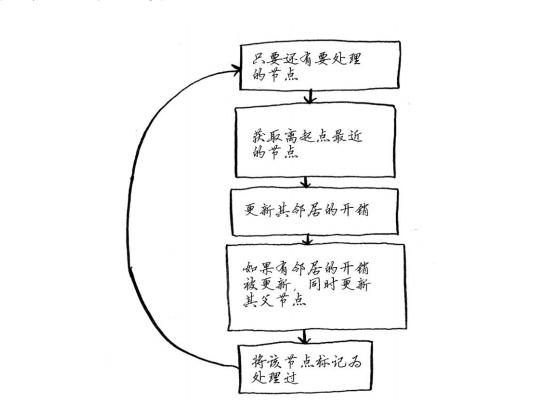
# 狄克斯特拉算法
四个步骤
- 找出最便宜的节点,即可在最短时间内前往的节点
- 对于该节点的令居,检查是否有前往他们更短路径,如果有,就更新其开销
- 重复这个过程,直到对图中每个节点都这么做了
计算非加权图的最短路径,使用广度优先搜索,计算加权图最短路径,使用迪科特斯拉算法。
创建一个表格,在其中列出每个节点的开销。这里的开销指的是达到节点需要额外支付多少钱。
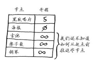
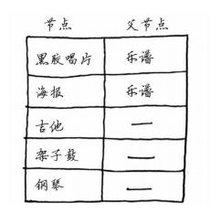
在执行狄克斯特拉算法的过程中,你将不断更新这个表。为计算最终路径,还需在这个表中添加表示父节点的列
如果有负权边,就不能使用狄克斯特拉算法。因为负权边会导致这种算法不管用。
计算方法
# the graph
graph = {}
graph["start"] = {}
graph["start"]["a"] = 6
graph["start"]["b"] = 2

graph["a"] = {}
graph["a"]["fin"] = 1

graph["b"] = {}
graph["b"]["a"] = 3
graph["b"]["fin"] = 5

graph["fin"] = {}

# the costs table
infinity = float("inf")
costs = {}
costs["a"] = 6
costs["b"] = 2
costs["fin"] = infinity

# the parents table
parents = {}
parents["a"] = "start"
parents["b"] = "start"
parents["fin"] = None

processed = []


def find_lowest_cost_node(costs):
    lowest_cost = float("inf")
    lowest_cost_node = None
    # Go through each node.
    for node in costs:
        cost = costs[node]
        # If it's the lowest cost so far and hasn't been processed yet...
        if cost < lowest_cost and node not in processed:
            # ... set it as the new lowest-cost node.
            lowest_cost = cost
            lowest_cost_node = node
    return lowest_cost_node


# Find the lowest-cost node that you haven't processed yet.
node = find_lowest_cost_node(costs)
# If you've processed all the nodes, this while loop is done.
while node is not None:
    cost = costs[node]
    # Go through all the neighbors of this node.
    neighbors = graph[node]
    for n in neighbors.keys():
        new_cost = cost + neighbors[n]
        # If it's cheaper to get to this neighbor by going through this node...
        if costs[n] > new_cost:
            # ... update the cost for this node.
            costs[n] = new_cost
            # This node becomes the new parent for this neighbor.
            parents[n] = node
    # Mark the node as processed.
    processed.append(node)
    # Find the next node to process, and loop.
    node = find_lowest_cost_node(costs)

print
"Cost from the start to each node:"
print(costs)

# result
# {'a': 5, 'b': 2, 'fin': 6}
广度优先搜索用于在非加权图中查找最短路径。 狄克斯特拉算法用于在加权图中查找最短路径。 仅当权重为正时狄克斯特拉算法才管用。 如果图中包含负权边,请使用贝尔曼福德算
# 近似算法
# You pass an array in, and it gets converted to a set.
states_needed = set(["mt", "wa", "or", "id", "nv", "ut", "ca", "az"])

stations = {}
stations["kone"] = set(["id", "nv", "ut"])
stations["ktwo"] = set(["wa", "id", "mt"])
stations["kthree"] = set(["or", "nv", "ca"])
stations["kfour"] = set(["nv", "ut"])
stations["kfive"] = set(["ca", "az"])

final_stations = set()

while states_needed:
  best_station = None
  states_covered = set()
  for station, states in stations.items():
    covered = states_needed & states
    if len(covered) > len(states_covered):
      best_station = station
      states_covered = covered

  states_needed -= states_covered
  final_stations.add(best_station)

print(final_stations)


## output
## {'ktwo', 'kone', 'kfive', 'kthree'}
贪婪算法寻找局部最优解,企图以这种方式获得全局最优解。 对于NP完全问题,还没有找到快速解决方案。 面临NP完全问题时,最佳的做法是使用近似算法。 贪婪算法易于实现、运行速度快,是不错的近似算法
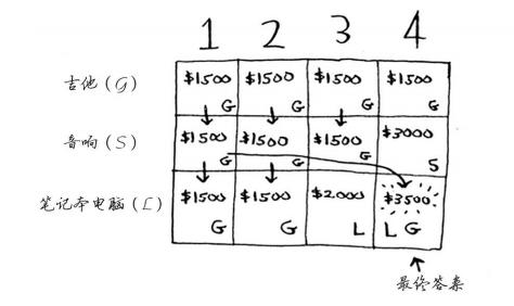
# 动态规划问题
动态规划从小问题着手,逐步解决大问题
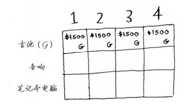
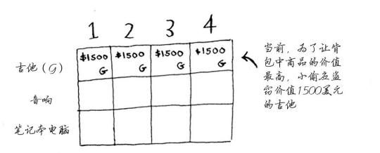
在每一行,可偷的商品都为当前行的商品以及之前各行的商品
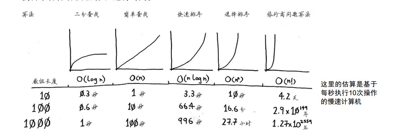
# o(1), o(n), o(logn), o(nlogn)的解释
在描述算法复杂度时,经常用到o(1), o(n), o(logn), o(nlogn)来表示对应算法的时间复杂度, 这里进行归纳一下它们代表的含义: 这是算法的时空复杂度的表示。不仅仅用于表示时间复杂度,也用于表示空间复杂度。
O后面的括号中有一个函数,指明某个算法的耗时/耗空间与数据增长量之间的关系。其中的n代表输入数据的量。
比如时间复杂度为O(n),就代表数据量增大几倍,耗时也增大几倍。比如常见的遍历算法。 再比如时间复杂度O(n^2),就代表数据量增大n倍时,耗时增大n的平方倍,这是比线性更高的时间复杂度。比如冒泡排序,就是典型的O(n^2)的算法,对n个数排序,需要扫描n×n次。 再比如O(logn),当数据增大n倍时,耗时增大logn倍(这里的log是以2为底的,比如,当数据增大256倍时,耗时只增大8倍,是比线性还要低的时间复杂度)。二分查找就是O(logn)的算法,每找一次排除一半的可能,256个数据中查找只要找8次就可以找到目标。 O(nlogn)同理,就是n乘以logn,当数据增大256倍时,耗时增大256*8=2048倍。这个复杂度高于线性低于平方。归并排序就是O(nlogn)的时间复杂度。 O(1)就是最低的时空复杂度了,也就是耗时/耗空间与输入数据大小无关,无论输入数据增大多少倍,耗时/耗空间都不变。
哈希算法就是典型的O(1)时间复杂度,无论数据规模多大,都可以在一次计算后找到目标(不考虑冲突的话)
# K 最近邻算法(K-nearestneighbours,KNN)
- 你需要对一个水果进行分类
- 查看他三个最近的令居
- 在这些令居中,橙子多于柚子,因此它很可能是橙子
余弦相似度: 实际工作中不使用距离公式,而是使用余弦相似度,不计算两个矢量的距离,而是比较他们的角度。
分类和回归
- 分类就是编组
- 回归就是预测结果(如一个数字)
# 二分查找树?
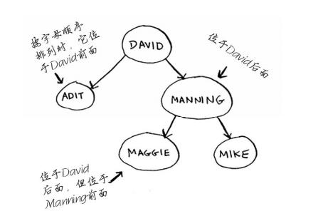
对于其中的每个节点,左子节点的值都比它小,而右子节点的值都比它大。
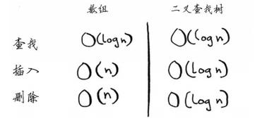
查找节点平均运行时间为 O(log n ) 最糟糕的情况下为 O(n) 在有序数组中查找时,即便是在最糟糕情况下也只有 O(log n ) 但是二分查找树插入和删除速度快很多
B树是一种特殊的二叉树,数据库常用它来存储数据。 待研究B树,红黑树、堆、伸展树
# 反向索引

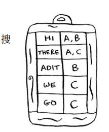
这个散列表的键为单词,值为包含指定单词的页面。现在假设有用户搜索hi,在这种情况下,搜索引擎需要检查哪些页面包含hi。 搜索引擎发现页面A和B包含hi,因此将这些页面作为搜索结果呈现给用户。现在假设用户搜 索there。你知道,页面A和C包含它。
# 布隆过滤器
布隆过滤器是一种概率型数据结构,它提供的答案有可能不对,但很可能是正确的
判断网页以前是否已搜集,可不使用散列表,而使用布隆过滤器。使用散列表时,答案绝对可靠,而使用布隆过滤器时,答案却是很可能是正确的
情况
- 可能出现错报的情况,即Google可能指出“这个网站已搜集”,但实际上并没有搜集。
- 不可能出现漏报的情况,即如果布隆过滤器说“这个网站未搜集”,就肯定未搜集
# HyperLogLog
HyperLogLog是一种类似于布隆过滤器的算法。
必须有一个日志,其中包含用户执行的不同搜索。有用户执行搜索时, Google 必须判断该搜索是否包含在日志中:如果答案是否定的,就必须将其加入到日志中
HyperLogLog近似地计算集合中不同的元素数,与布隆过滤器一样,它不能给出准确的答案,但也八九不离十,而占用的内存空间却少得多
# SHA算法
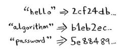
散列函数是安全散列算法(secure hash algorithm, SHA)函数。给定一个字符串, SHA返回其散列值。
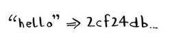
SHA是一个散列函数,它生成一个散列值——一个较短的字符串。用于创建散列表的散列函数根据字符串生成数组索引,而SHA根据字符串生成另一个字符串
文件对比:
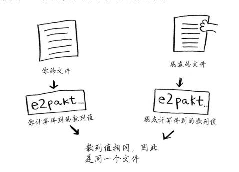
散列算法是单向的
SHA实际上是一系列算法: SHA-0、 SHA-1、 SHA-2和SHA-3。本书编写期间, SHA-0和SHA-1 已被发现存在一些缺陷。如果你要使用SHA算法来计算密码的散列值,请使用SHA-2或SHA-3。 当前,最安全的密码散列函数是bcrypt,但没有任何东西是万无一失的。
# Simhash 算法
Simhash生成的散列值也只存在细微的差别。这让你能够通过比 较散列值来判断两个字符串的相似程度
- Google使用Simhash来判断网页是否已搜集。
- 老师可以使用Simhash来判断学生的论文是否是从网上抄的。
- Scribd允许用户上传文档或图书,以便与人分享,但不希望用户上传有版权的内容!这个网站可使用Simhash来检查上传的内容是否与小说《哈利·波特》类似,如果类似,就自动拒绝。
# Diffie-Hellman 和 RSA
Diffie-Hellman使用两个密钥:公钥和私钥。顾名思义,公钥就是公开的,可将其发布到网站上,通过电子邮件发送给朋友,或使用其他任何方式来发布。你不必将它藏着掖着。有人要向你发送消息时,他使用公钥对其进行加密。加密后的消息只有使用私钥才能解密。只要只有你知道私钥,就只有你才能解密消息!
替代者 :RSA